Rethinking Asset Valuation in a Competitive Environment[1]
By Rajat Deb LCG Consulting
As restructuring gains
momentum, and both power plant acquisitions and new generator investments take
on greater strategic significance, the use of forward prices of electricity for
asset valuation has become common. Since expected revenues and profits are
central elements in such capital decisions, it is worth examining whether
methods used to calculate forward price curves meet certain basic conditions.
First, do the relevant calculations include all products that the asset's
revenue will depend upon? Do they meaningfully incorporate those rare
events having large price effects over an extended time horizon? These
questions go to the heart of whether a method is either appropriate or adaptive
to asset valuation in the future electricity market.
When the forward price
curve is focused solely on energy, the assumption is made that generators would
passively accept whatever price the forward energy market offers, exclusive of
other markets. In practice, a generator operator will seek to maximize
income by seeking profits and advantage across all available markets. In
order to reveal the full earnings potential of the asset, valuation must also
include the revenues that operators will earn from proactive participation in
the lucrative ancillary service and spot markets. The price risk that
characterizes power markets is too considerable to suppose that market
participants will not continuously compare the levels of profit potentially
available in the various product markets.
Black's Model: Not practical for Multiple Bids
The most commonly used
forward-price method is relatively simple in concept. To determine the
earnings potential of a base-loaded unit like a combined cycle (CC) unit, the
NPV (net present value) of the spark spread (the difference between the forward
price and the variable operating cost of the unit) is calculated and aggregated
over its lifetime. For cycling units like combustion turbines, the
calculation is similar to that used for the CC, except an annual price duration
curve is occasionally used to capture the cycling behavior of the unit.
The price duration curve allows a quick appraisal of those hours during which a
CT can and should profitably operate; a CC is assumed to serve base-load
capacity at all hours, less those lost to outages, due to its lower costs.
In either case, the method by which the forward price curve is obtained is the
key to the investment decision.
In attempts to develop
forward price curves, projections using a Black’s model-type analysis are
sometimes used. While the past may be used as a guide to the current
behavior of standardized commodity prices however, the electricity market is
distinguished by its current evolution and its tremendous short-term, intra-hour
volatility. Historical methods lack justification in that they do not meet
the two conditions put forth earlier - inclusion of potential revenues from
multiple products and markets, and incorporation of rare events causing price
spikes.
The
period in which energy was a monolithic product is now past. Recently,
California, ISO-NE (the former NEPOOL), and PJM have established more clearly
than ever before a distinction between energy, ancillary services and reserve
capacity products. The new product markets, as well as the spot markets in
energy, offer alternative sources of revenue to the forward energy market.
Their prices will depend on the energy market, and vice versa, with the
exhaustion of arbitrage opportunities acting nominally, at least, to constrain
unlimited inter-market basis differences.
Due to
the ongoing restructuring in major regional markets, historically derived
analyses are necessarily based on scant data and are faced
with a lack of liquidity in multiple markets. Black’s model, in order to
incorporate ancillary services, would require analyzing liquid futures in
multiple commodity markets, not just those in energy. Moreover, those
commodity prices and quantities that would characterize liquid energy and
ancillary services markets would be highly correlated, whereas Black's model is
not capable of application across multi-product markets.
Price Spikes: Not Captured in Most Methods
As concerns price
spikes, an historical model can not capture the instantaneous supply-demand
equilibration which occurs continuously in electricity, and which introduces the
characteristic volatility of spot or imbalance prices. (Given the variety
of factors that affect electricity prices, even the spark spread, or basis
difference between prices of gas and electricity, fluctuates with unpredictable
frequency and magnitude.) The factors behind price spikes, and the
concurrence of extreme, unpredictable events in terms of precise weather, system
outage patterns, and/or demand conditions are not likely to follow historical
occurrences. Thus, deriving a future dependency through regression is full
of uncertainty, and invites the superposition of one source of volatility upon
another.
An alternative to the
historical approach merits attention, for the strengths it offers in the same
areas in which historical projections suffer their most serious weaknesses.
A Multi-product, Multi-area Optimal Power Flow model (MMOPF) model with
real-time dispatch is a structural model that incorporates generation, load and
transmission data into a dynamic simulation. Such a structural model
is required to simulate the hourly price
fluctuations, and to ascertain how the uncertain distribution of the fundamental
price drivers affects the price distributions among markets. (A description of
such models can be found in [[2]].)
Such a structural model performs these analyses by its fusion of the
technological characteristics of plants, their operational choices and market
eligibility, and by incorporating the system constraints which affect the
real-time dispatch of generating units. Fuel prices, demand fluctuation
and emergency outages are some of the elements that are combined with overall
system conditions within a structural model.
As for the
introduction of new technologies, valuation with a structural model can also
project the actual market participation by a unit, given its relevant
characteristics and bid parameters. The range of product markets available
to combustion turbines is especially broad, and thus ancillary services will
make up a relatively larger portion of overall revenue than they will for other
generators. Even if a plant is only able to provide energy, its valuation
needs to take into account the interaction of prices in forward, spot, and
ancillary services markets.
A structural model
makes possible volatility analysis, which captures the systematic effects of key
driver distributions and interactions. By running multiple scenarios based
on Monte Carlo sampling of the distributions of fundamental market drivers, one
can obtain the volatility distribution of both energy and ancillary service
prices. The drivers’ distributions are changeable, given new information
or a need to explore scenarios under changed conditions.
Whereas a time-series
model will not be able to account for the occurrence of price spikes, a
structural model can derive a reasonable estimate of their likelihood, given the
coincidence of less likely values among key drivers over multiple scenarios.
For a long-term structural simulation, the number, severity and duration of
price spikes will all result from the other system conditions encompassed by the
model. Indeed, price spikes may provide crucial revenue to enable a
plant's profitable operation. In asset valuation, insights into these
phenomena can prove decisive.
Most importantly, a
structural approach offers the ability not only to capture the prices in the
electricity markets based on rational bidding by participants, but incorporates
the dynamic interaction of prices in the various markets.
A Case Study: Simultaneous Bidding in Multiple markets
An illustration of the
impact of earning revenues from multiple product markets will follow. We
use a MMOPF-type model to derive the revenues of individual CC and CT units
whose characteristics are displayed in Table 1.
Table 1. Characteristics of Generating Assets
|
|
Combined Cycle Unit
|
Combustion Turbine
|
|
Unit Size (MW)
|
400
|
200
|
|
Heat Rate (Mbtu/MWh)
|
6700
|
8500
|
|
Fuel Cost ($/Mbtu)
|
2.1
|
2.1
|
|
Start-up Cost ($/MW)
|
30
|
20
|
|
Day-ahead* Cost ($/MWh)
|
17.49
|
20.52
|
|
Marginal Cost
|
15.07
|
17.85
|
|
Fixed O&M Cost ($kW-Yr)
|
18
|
12
|
|
*Includes One Start-up & $1/MWh Variable O&M
|
Asset valuation results based on the forward price curve of energy will be
compared with the units’ earnings when they are bid into the ancillary services
and spot markets. The model outputs used are prices for energy, regulation
up, regulation down, spinning and non-spinning reserves, replacement reserve and
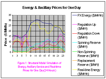
real-time, all of which are displayed in Table 2 and shown in Figure 1 for a
particular day.
What happens if plants bid only on one product, in the day-ahead market for
energy in the power exchange?
Energy Only
First, the forward curve is used to derive purely forward energy market-based
revenues. Note that from Table 1, the marginal cost of the CC is $15.07.
In the day-ahead PX market, a bid of $0 will allow the generator to be
dispatched in every hour, and obtain revenue over marginal cost in most hours.
It is better for the generator to incur a small loss for a few hours than to pay
the additional start-up cost that would be necessitated after shutting down
briefly.
Table 2. MMOPF simulation of day-ahead forward, ancillary services and real-time prices.
|
Hour
|
PX Energy ($/MWh)
|
Reg Up ($/MW)
|
Reg Down ($/MW)
|
Spinning Reserve ($/MW)
|
Non-Spinning Reserve ($/MW)
|
Replace-ment Reserve ($/MW)
|
Real-time energy ($/MWh)
|
Optimal Bid for CC
|
|
PX Energy Bid
|
Regulation Bid
|
|
1
|
16.19
|
10.31
|
6.88
|
3.00
|
2.19
|
0.00
|
9.87
|
25.38
|
1.12
|
|
2
|
15.73
|
15.44
|
10.29
|
2.00
|
0.57
|
0.00
|
10.98
|
30.51
|
0.66
|
|
3
|
14.57
|
15.94
|
10.63
|
0.00
|
1.01
|
0.00
|
12.02
|
31.01
|
0.00
|
|
4
|
13.55
|
14.73
|
9.82
|
0.00
|
0.63
|
0.00
|
10.55
|
29.80
|
0.00
|
|
5
|
13.57
|
6.34
|
4.23
|
0.00
|
0.21
|
0.00
|
9.45
|
21.41
|
0.00
|
|
6
|
15.56
|
15.34
|
10.22
|
3.00
|
0.73
|
0.00
|
8.67
|
30.41
|
0.49
|
|
7
|
17.58
|
16.45
|
10.96
|
4.00
|
0.45
|
0.00
|
13.25
|
31.52
|
2.51
|
|
8
|
22.03
|
7.22
|
4.81
|
5.00
|
2.03
|
0.00
|
12.56
|
22.29
|
6.96
|
|
9
|
28.01
|
6.01
|
4.00
|
5.00
|
4.01
|
0.00
|
25.34
|
21.08
|
12.94
|
|
10
|
28.68
|
4.10
|
2.73
|
6.00
|
4.68
|
0.00
|
28.03
|
19.17
|
13.61
|
|
11
|
30.76
|
4.29
|
2.86
|
8.00
|
4.76
|
1.00
|
27.22
|
19.36
|
15.69
|
|
12
|
30.83
|
4.85
|
3.24
|
8.00
|
4.83
|
2.03
|
27.78
|
19.92
|
15.76
|
|
13
|
30.15
|
6.28
|
4.19
|
8.00
|
4.15
|
2.01
|
22.33
|
21.35
|
15.08
|
|
14
|
28.20
|
6.05
|
4.04
|
10.00
|
4.09
|
2.68
|
22.00
|
21.12
|
13.13
|
|
15
|
27.57
|
9.28
|
6.19
|
10.00
|
4.47
|
2.76
|
22.76
|
24.35
|
12.50
|
|
16
|
27.23
|
11.53
|
7.69
|
12.00
|
4.22
|
2.83
|
18.13
|
26.60
|
12.16
|
|
17
|
27.01
|
11.85
|
7.90
|
12.00
|
4.75
|
2.15
|
18.15
|
26.92
|
11.94
|
|
18
|
27.00
|
9.98
|
6.65
|
10.00
|
4.63
|
2.09
|
20.16
|
25.05
|
11.93
|
|
19
|
24.12
|
8.81
|
5.88
|
10.00
|
4.69
|
2.47
|
24.75
|
23.88
|
9.05
|
|
20
|
23.62
|
9.38
|
6.25
|
11.00
|
4.63
|
2.22
|
24.82
|
24.45
|
8.55
|
|
21
|
24.06
|
12.95
|
8.64
|
7.00
|
4.59
|
2.75
|
24.00
|
28.02
|
8.99
|
|
22
|
22.15
|
17.49
|
11.66
|
5.00
|
4.15
|
2.63
|
23.16
|
32.56
|
7.08
|
|
23
|
17.73
|
14.84
|
9.89
|
5.00
|
2.73
|
2.59
|
18.90
|
29.91
|
2.66
|
|
24
|
16.54
|
9.92
|
6.62
|
2.00
|
0.54
|
0.00
|
18.35
|
24.99
|
1.47
|
|
Daily Average Price
|
22.6
|
10.39
|
6.93
|
5.99
|
3.07
|
1.43
|
18.88
|
|
|
According to the overall market-clearing operations, and as indicated in Figure
1, the price of energy will be above the CC's marginal cost for 21 hours.
Thus, the CC will earn an income of $181/MW-Day.
The daily income
changes with forward prices, and the total income over the initial and
subsequent years adds up to $78,277/MW-Year. The NPV of the income
generated over the unit's lifetime is $638/kW. The corresponding numbers
for the CT are $94/MW-Day, $29,333/MW-Year and $177/kW, respectively.
These earnings are
based on the expected annual earnings for the unit, taking into consideration
the impact of outages, seasonal price volatility, and operational costs.
Ancillary Services
A CC plant, when equipped with AGC (automatic generation control), can
participate in the regulation market. If selected for regulation, a unit
is paid to maintain capacity and is dispatched as needed by the ISO. In
California's current market structure, availability payments are not withdrawn
when a unit is paid for dispatch. Rather, the two payments overlap.
In order to develop
bids, the operator needs a set of expectations regarding the prices from the
energy and ancillary services markets like those in Figure 1.
From these
prices, a bidding strategy can be developed. Thus, the maximum possible
profit based on expected prices in various markets within each hour is given in
Figure 2.
Glancing from the profit trend in Figure 2 to Figure 1, one will see that the
generator’s highest expected profits in the early and late hours of the day lie
in the regulation up market. During peak hours, the higher PX energy
prices promise the most profit in that market.
In addition to the income from energy and regulation up availability, Figure 2
displays a potential revenue trend called “supplemental real-time income.”
It indicates the net income that would result whenever a generator were required
to supply energy by the ISO. The hourly
income is given by the hourly real-time energy price, which is what the
generator receives, less marginal cost.
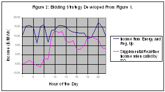
The dispatch revenue is called “supplemental” in this discussion because the
ancillary service reserves the unit, but cannot guarantee energy production in
terms of capacity or duration of operation. It therefore carries some
uncertainty.
If the CC unit in the example were dispatched for
real-time energy during the hours when it is supposed to provide ancillary
service, a net loss could be incurred during the early hours, while positive net
revenue would be earned in the latter part of the day. Since the
proportion of the generator’s capacity that can be dispatched for ancillary
service purposes is a part of (never more than) the total capacity secured
through availability payments, the availability payments will have greater
magnitude than dispatch income in the overall profit calculation. The
percentage of capacity that will actually be dispatched will vary according to
the type of service and fluctuation in the need for it.
How should a bidding strategy balance the various simultaneous profit opportunities in multiple product markets?
Balancing Profit Potential
The operator of this unit needs a bidding strategy that will result in a uniform
expected level of profit, whichever market accepts him. The rationale
behind this condition is the optimization of income, assuming indifference to
the origin of profit. Given the expectations summarized in Figures 1 and 2, the
operator develops bids that position the generator as a price-taker in the most
profitable market during each hour. Clearly, the priority for an
AGC-equipped generator would be to enter the energy market at peak hours, and to
be scheduled for regulation availability during off-peak hours. A
generator unable to serve regulation would need to consider the next most
profitable market after regulation, spinning reserve, if the generator were
capable.
In the off-peak hours,
the bids into the regulation up market would be the expected energy price less
its marginal cost (as regulation carries no marginal cost). His regulation
bids are low enough to have a high likelihood of acceptance. Thus, he
stands to make no less from regulation than the expected energy market profit.
As explained, the operator should bid to insure the same profit across markets,
that is, whatever the most profitable market promises. The corresponding
hourly bid into the PX for energy should be the marginal cost of delivery plus
the expected regulation profit, which is regulation’s expected price.
Bids and Earnings
Suppose the operator expects the clearing price for regulation availability will
be $10.00/MWh. The marginal cost of the CC in our example to supply energy
is $15.07/MWh, so to equalize his profit
across markets, he bids $25.07/MWh (=15.07 + 10.00), into the PX. Thus, a
minimum profit of $10.00 from energy would result from acceptance, commensurate
with the profit expected through regulation.
During peak hours,
when energy is expected to offer the highest profit, his bid into the forward
energy market is the expected regulation price (also the expected regulation
profit) plus the marginal cost of generation ($15.07). The rational bid
for regulation is the profit expected from energy, or the anticipated energy
price less the marginal cost (again, because regulation carries no marginal
cost).
On the basis of its
bidding strategy, the AGC-equipped CC in this example is scheduled for dispatch
in the energy market for 11 consecutive hours, 9 through 19. For the other
13 hours of the day, it is scheduled for regulation up availability, and will be
running at a minimum level, to be dispatched as needed by the ISO. The
profit that the unit makes in each market is calculated below.
The resultant energy
earnings are the summation of the difference between the market-clearing PX
energy price and the marginal cost for the 11 hours just stated, times 400 MW
(the unit’s capacity). The earnings for regulation up availability are
given by the summation of the market-clearing regulation up prices in hours 1
through 8, and 20 through 24, times 400 MW of capacity accepted. Dispatch
by the ISO for regulation will supplement the income. For the revenue
calculation in this example, 40 MW is needed during all 13 hours of regulation,
and the real-time energy price is paid per MWh. Thus, the revenue from
real-time dispatch for regulation can be calculated as the summation of
differences between the real-time energy prices and marginal cost for the 13
stated hours of dispatch, times 40 MW.
Table 3.Bid prices and incomes for the CC
and CT units for one day of operation in PX/ISO market protocol
(Note: Regulation down, Spinning reserve, and Replacement are omitted,
as no revenue accrued to the generator for these services.)
|
|
PX Energy ($/MWh)
|
Regulation Up ($/MW)
|
Non-Spinning Reserve ($/MW)
|
Real-time Energy ($/MWh)
|
|
Revenue of the CC Unit
|
|
Bid Price ($/MWh)
|
24.00
|
0.00
|
|
|
|
Hours Exercised
|
11
|
13
|
|
13
|
|
Income ($/MWh)
|
13.07
|
12.8
|
|
0.05
|
|
Revenue of the CT Unit
|
|
Bid Price ($/MWh)
|
26.00
|
|
0.00
|
|
|
Hours Exercised
|
10
|
|
14
|
|
|
Income ($/MWh)
|
8.02
|
|
2.08
|
|
The income the unit
has achieved after bidding into the PX and ancillary services markets is
$310/MW-day. These results are summarized in Table 3. The daily and annual
earnings and the NPV over the lifetime of the unit are given in Table 4.
Table 4.Daily, annual and NPV of Income
|
|
Revenue Based on Conventional Operation |
Revenue Based on Proactive Participation in all Markets |
|
Combined Cycle Price Taker |
CT Marginal Cost Bid |
Combined Cycle |
Combustion Turbine |
|
One-Day Income ($/MW-Day) |
181 |
94 |
310 |
109 |
|
Annual Income ($/MW-Yr) |
78,277 |
29,338 |
108,335 |
40,670 |
|
NPV of Lifetime Income ($/kW) |
638 |
177 |
883 |
246 |
In the case of the
combustion turbine, the bid for energy is marginal cost plus the clearing price
of non-spinning reserve prices. From Table 3, one can see that the unit
participates for 10 hours in the energy market and for 14 hours in the
non-spinning reserve market. The daily and annual net incomes are
illustrated in Table 4. The net present value (NPV) represents the
summation of these values over the lifetime of the asset. Note that the
unit earns $246/kw, rather than the $177/kW shown in the case of conventional
analyses.
A comparison of the
two units’ valuations, the first based on energy alone and the other on multiple
product bidding (shown in Table 4), suggests the sort of error that one invites
with historical projections based on energy. These examples show that with
a rational, profit-optimizing approach such as that outlined, a generator can
gain access to greater overall revenues. The simplistic assumption that,
over its lifetime, a unit will participate in the energy market and may even
receive some capacity charges may underestimate its potential income. In
California, New England, New York, PJM and Ontario, there is a definite
advantage to participating in ancillary service and spot markets, where active
ancillary services and real-time imbalance bidding is in place.
Regional Markets: All Equally Friendly?
The task of asset valuation requires attention to the type of ancillary service
markets in the relevant region and according to the market structure in place. For instance, ECAR does not have a bidding system for distinct ancillary
service products, but is divided between energy and capacity payments. The operation of ancillary services markets in California
thus far has seen fewer bids than are necessary to meet ISO requirements for
ancillary services, and has removed some supply-side incentive to broader
participation through the imposition of price caps. Despite the progress that lies ahead in the emergence of liquid ancillary
services markets, generators’ operational characteristics, and their competitive
positioning in providing various products requires scrutiny. The price of energy is insufficient to provide an estimate of a generator's
worth. If it alone is used in revenue forecasts,
such forecasts are likely to make generators with different technologies appear
more similarly profitable than they may actually prove to be. As operators gain insight concerning the prices prevalent in a particular
market, their minimum requirements for return from other markets will inevitably
cause dynamic price changes. For different generator
technologies, the various price fluctuations will affect the temporal bidding
profile they adopt.
While appropriate for an environment dominated by regulatory price determination
for a single product, the forward price curve of electricity needs to be
augmented in order to conduct strategic planning in the emerging competitive
environment. The model based on single-commodity pricing necessarily ignores the
possibility for generators’ strategic, multiple product bids and the timing of
units’ dispatch opportunities, linked to start-up costs and minimum run
duration. In sum, the old approach leaves the income
from ancillary services and supply imbalances out of the resultant valuation
entirely. Hence, a structural model with the ability to capture price volatility
and dynamic interaction for all products is needed to provide an internally
consistent set of price curves, and base the earnings from respective sources on
the dispatch. In this way, we now can provide a comprehensive assessment of generator
value that properly incorporates multiple products and markets[3].
_________________________________________________